The weird, biased wisdom of the crowd

Here’s the tweet that announced the contest:

Data science CONTEST!

A lab member told me that a class he was in came extremely close to guessing how many candies in the jar–if the mean of guesses was taken as the answer

Go!

*Analysis, correct answer after replies come in. See my skittlecytometer for counting method 👇 pic.twitter.com/1kqUHJzYNG

— J. Brian Byrd, MD, MS 🐦 (@thebyrdlab) August 27, 2019

Shortly after I shared the contest, @drnic1 shared a 1980’s publication on visual estimation tasks and economics.

@DavidSFink went even futher into the archives to show that Francis Galton wrote about estimation and the wisdom of the crowd in Nature in 1907.

The framing of Galton’s article was whether the populace can be trusted to have good political judgment.

This actually is much older than any economic experiment, but dates back to Sir Francis Galton https://t.co/FxI87IANLT

— David Fink (@DavidSFink) August 27, 2019

The summary of the Galton article is that about 800 people guessed the weight of an ox at the West of England Fat Stock and Poultry Exhibition.

The crowd in Galton's paper pretty much nailed it. The middlemost estimate was only 0.8 percent from the actual weight.

Returning to today’s contest, let’s take a look at the guesses tweeps provided.

First, we need to load the relevant R packages and the data, with a quick check for duplicates.

require(readxl) # Load package to import the data from Excel file
require(lubridate) # Load package that converts unusual Twitter-format date-times to R-friendly POSIXct
require(ggplot2) # Load data visualization packages
require(dplyr) # Load libray used in analysis
guessDf <- read_excel("/Users/jbrianbyrd/Box Sync/Byrd Backup Files/Data/Data_Science_Contest/Guesses.xlsx") # Import contest data
# Check for duplicates
duplicated(guessDf$tweepHandle)

##  [1] FALSE FALSE FALSE FALSE FALSE FALSE FALSE FALSE FALSE FALSE FALSE
## [12] FALSE FALSE FALSE FALSE FALSE FALSE FALSE FALSE FALSE FALSE FALSE
## [23] FALSE FALSE FALSE FALSE FALSE FALSE FALSE FALSE FALSE FALSE FALSE
## [34] FALSE FALSE FALSE FALSE FALSE FALSE FALSE FALSE FALSE FALSE FALSE
## [45] FALSE FALSE FALSE FALSE FALSE FALSE FALSE FALSE

Let’s now deal with Twitter’s unusual date format, using the ‘subst’ function to extract the date and the time in R and the ‘lubridate’ package to create a standard-format date-time.

# Extact the date of contest entries fom the Twitter-formatted date-times
guessDf$rFriendlyDate<-substr(guessDf$twitterFormatTimeDate,11,23)
# Extact the time of contest entries fom the Twitter-formatted date-times
guessDf$rFriendlyTime<-substr(guessDf$twitterFormatTimeDate,1,8)
# Use lubridate to convert dates and times to a POSIXct date-time value
guessDf$rFriendlyDateTime = mdy_hm(paste(guessDf$rFriendlyDate, guessDf$rFriendlyTime))

Data loading and cleaning behind us, let’s start analyzing the contest results.

We need to know how far each person’s guess was from the true answer.

# Calculate distance between tweeps' guess and correct count
guessDf$guessDistance<-guessDf$guess-723

Let’s plot all the guesses I received in terms of their distance from the correct count.

# Plot the guess distances by tweep handle
guessDf$guessType <- ifelse(guessDf$guessDistance < 0, "below", "above")  # above / below avg flag
guessDf <- guessDf[order(guessDf$guessDistance), ]  # sort
guessDf$tweepHandle <- factor(guessDf$tweepHandle, levels = guessDf$tweepHandle)  # convert to factor to retain sorted order in plot.
# Plot guess distance
theme_set(theme_bw())
ggplot(guessDf, aes(x=tweepHandle, y=guessDistance, label=guessDistance)) + 
  geom_point(stat='identity', aes(col=guessType), size=6)  +
  scale_color_manual(name="Guess", 
                     labels = c("Too High", "Too Low"), 
                     values = c("above"="#00ba38", "below"="#f8766d")) + 
  geom_text(color="white", size=2) +
  labs(title="Guess Distance from Correct Answer",y="Guess Distance", x="Tweep Handle") + 
  coord_flip()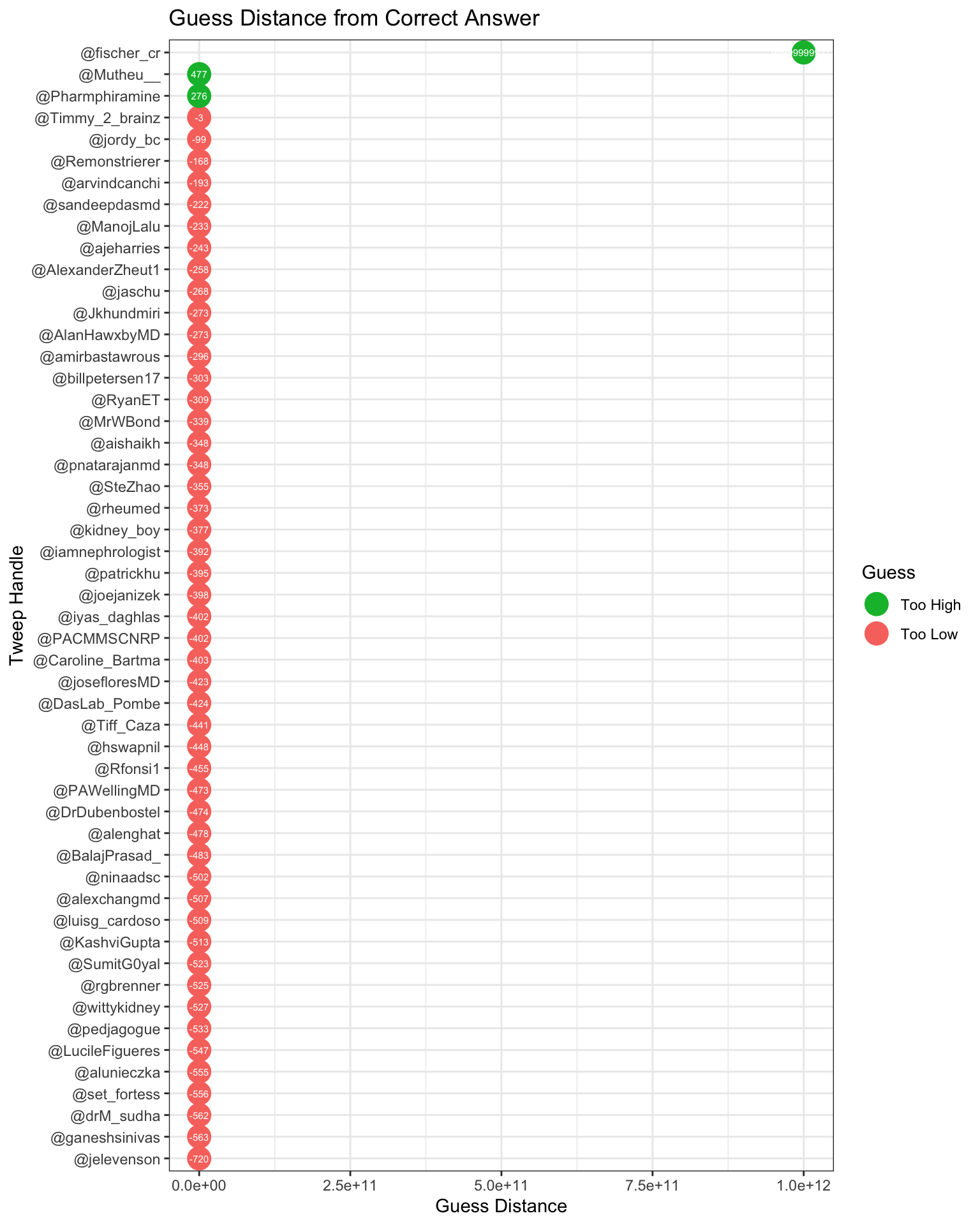

Ok, you can see a problem. @fischer_cr wanted to keep me on my toes in terms of data visualization, so he guessed 1 trillion.

Just because I want to see how you average these guesses, I want to register my guess of ONE TRILLION

— Curt Fischer (@fischer_cr) August 31, 2019

Also, @jelevenson–whom I know from working with him when he was a fantastic resident–guessed 3.

1, 2, …. 3. 3! pic.twitter.com/nKOItOzX2N

— Joshua Levenson, MD (@jelevenson) August 30, 2019

Since these guesses were amusing more than informative, I removed them from the dataset. Let’s try again.

# Remove joke guesses
guessDf<-guessDf[guessDf$guess!=3 & guessDf$guess!=1000000000000, ]
# Plot guess distance for non-joke guesses
theme_set(theme_bw())
ggplot(guessDf, aes(x=tweepHandle, y=guessDistance, label=guessDistance)) + 
  geom_point(stat='identity', aes(col=guessType), size=6)  +
  scale_color_manual(name="Guess", 
                     labels = c("Too High", "Too Low"), 
                     values = c("above"="#00ba38", "below"="#f8766d")) + 
  geom_text(color="white", size=2) +
  labs(title="Guess Distance from Correct Answer",y="Guess Distance", x="Tweep Handle") + 
  coord_flip()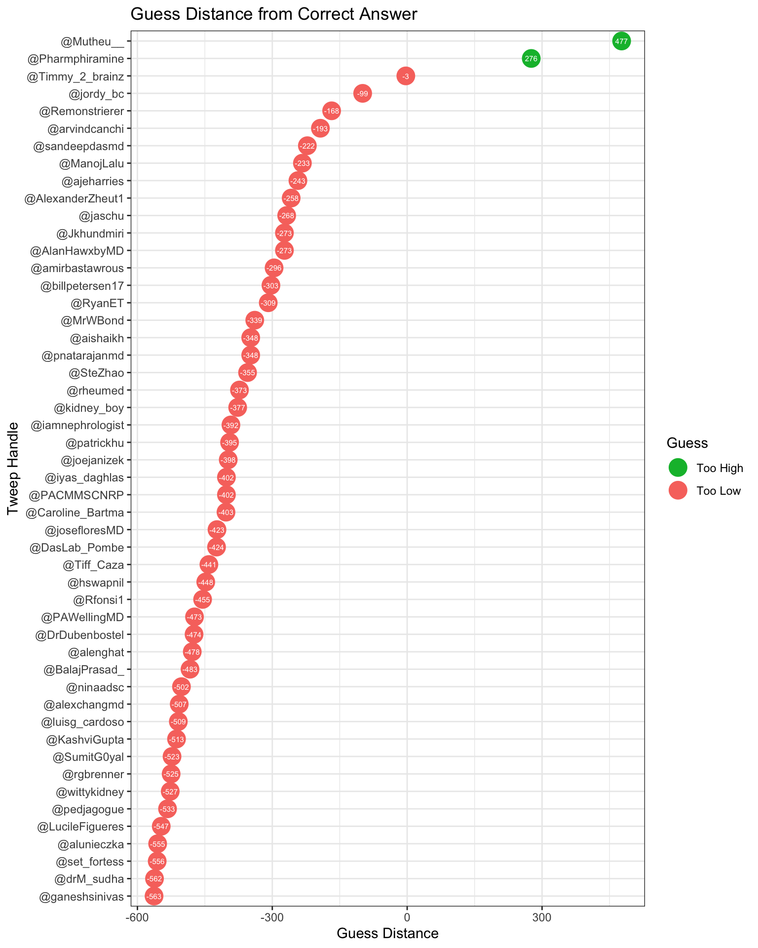

It’s pretty clear who won, but let’s verify who the winner is.

# Calculate the absolute value of the guess distance
guessDf$absGuessDistance<-abs(guessDf$guessDistance)
# Find the minimum absolute value among the guess distances
min(guessDf$absGuessDistance)

## [1] 3

# Find the index of the entry with the smallest guess distance
guessDf %>% 
  slice(which.min(absGuessDistance))

## # A tibble: 1 x 9
##   guess tweepHandle twitterFormatTi… rFriendlyDate rFriendlyTime
##   <dbl> <fct>       <chr>            <chr>         <chr>        
## 1   720 @Timmy_2_b… 9:03 PM · Aug 3… Aug 30, 2019  "9:03 PM "   
## # … with 4 more variables: rFriendlyDateTime <dttm>, guessDistance <dbl>,
## #   guessType <chr>, absGuessDistance <dbl>

Congratulations to @Timmy_2_Brainz, the winner of the contest!

As you can see from the above lollipop plot, he was only 3 away from the true count.

I promised to send a Galton board https://galtonboard.com/ to the winner, and I plan to do so after I verify that having 2 brains isn’t a rule violation.

@Timmy_2_Brainz was off by only 0.41%! I am wondering whether he estimated visually, or calculated his answer*

*Thank you, @AdamAkers18 for alerting me to the Kepler conjecture and Thomas Hales’ proof of it https://en.wikipedia.org/wiki/Kepler_conjecture.

(abs(720-723))/723*100

## [1] 0.4149378

So the winner pretty much nailed it, but the wisdom of the crowd in estimation tasks has been thought to be a function of everyone’s guess, not an individual’s.

Let’s look at how the guesses look from smallest to largest

# Quantiles for guesses
guessDf$fraction<-(1:length(guessDf$guess) - 1)/(length(guessDf$guess) - 1)
ggplot(guessDf, aes(fraction, sort(guess))) + 
  geom_point() + geom_line() + labs(main = "Quantiles for Guesses", x = "Sample Fraction", y = "Sample Quantile")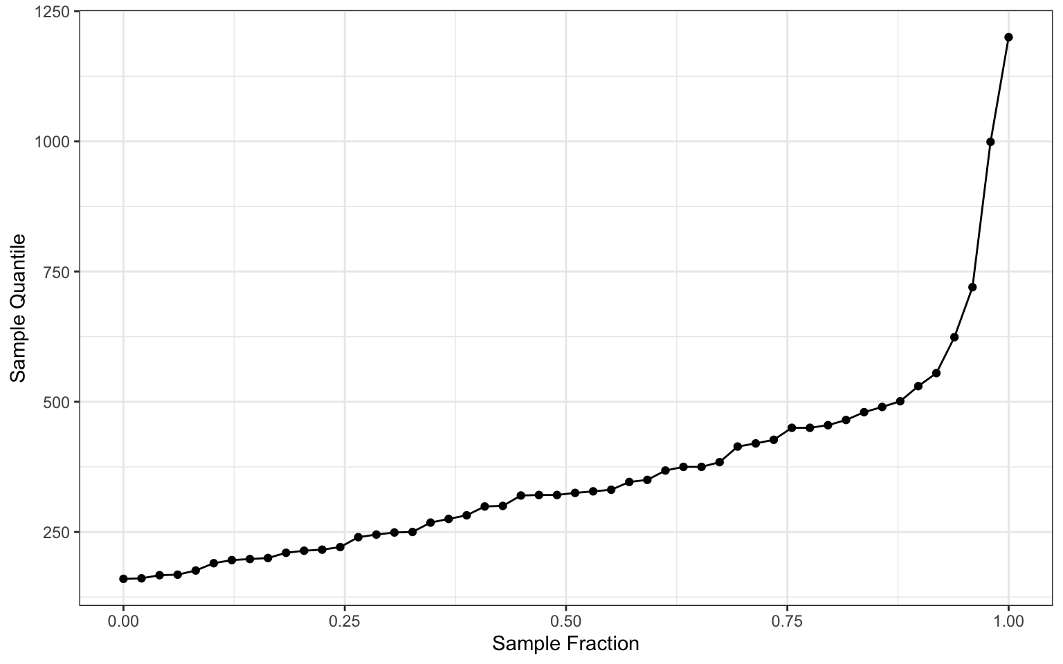

Here is the histogram of responses. By now, you’re probably noticing that the guesses were not normally distributed.

# Histogram of guesses
ggplot(guessDf, aes(guess)) + geom_histogram() + labs(x="Guess",y="Count") + geom_vline(xintercept = 723, linetype="dashed", 
                                                                                        color = "blue", size=1) + geom_text(x = 850,y = 5, label="True Count (723)")

## `stat_bin()` using `bins = 30`. Pick better value with `binwidth`.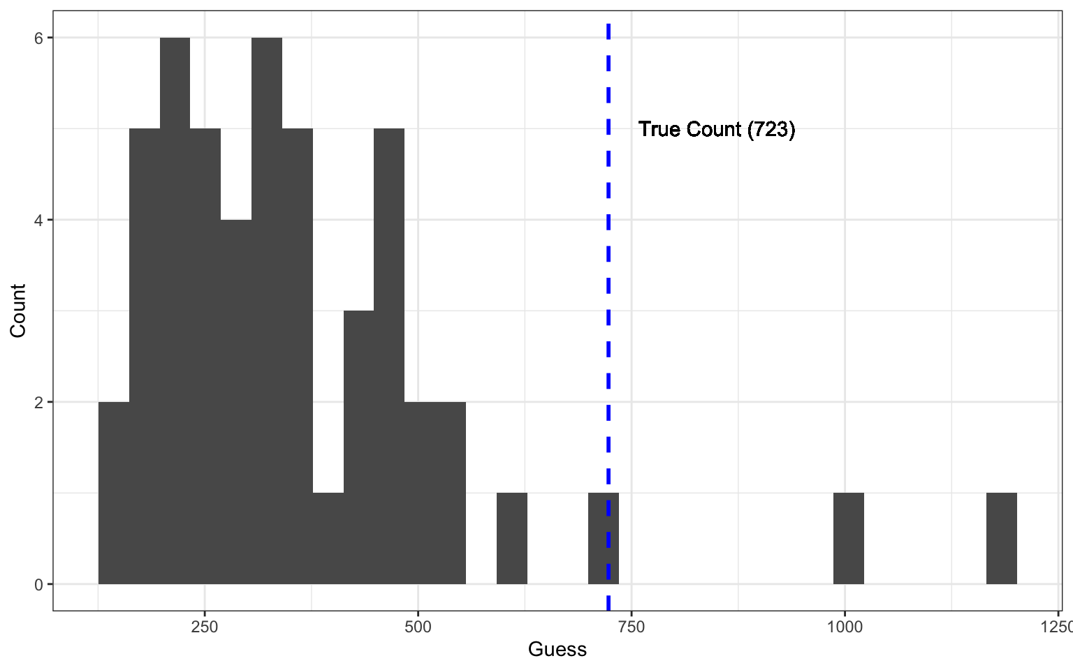

To look at the non-normality of the data in a second light, here is a quantile-quantile plot comparing the quantiles of the observed data to quantiles of normally distributed data.

# Quantile-quantile plot of observations and normal distribution
p <- ggplot(guessDf, aes(sample = guess))
p + stat_qq() + stat_qq_line()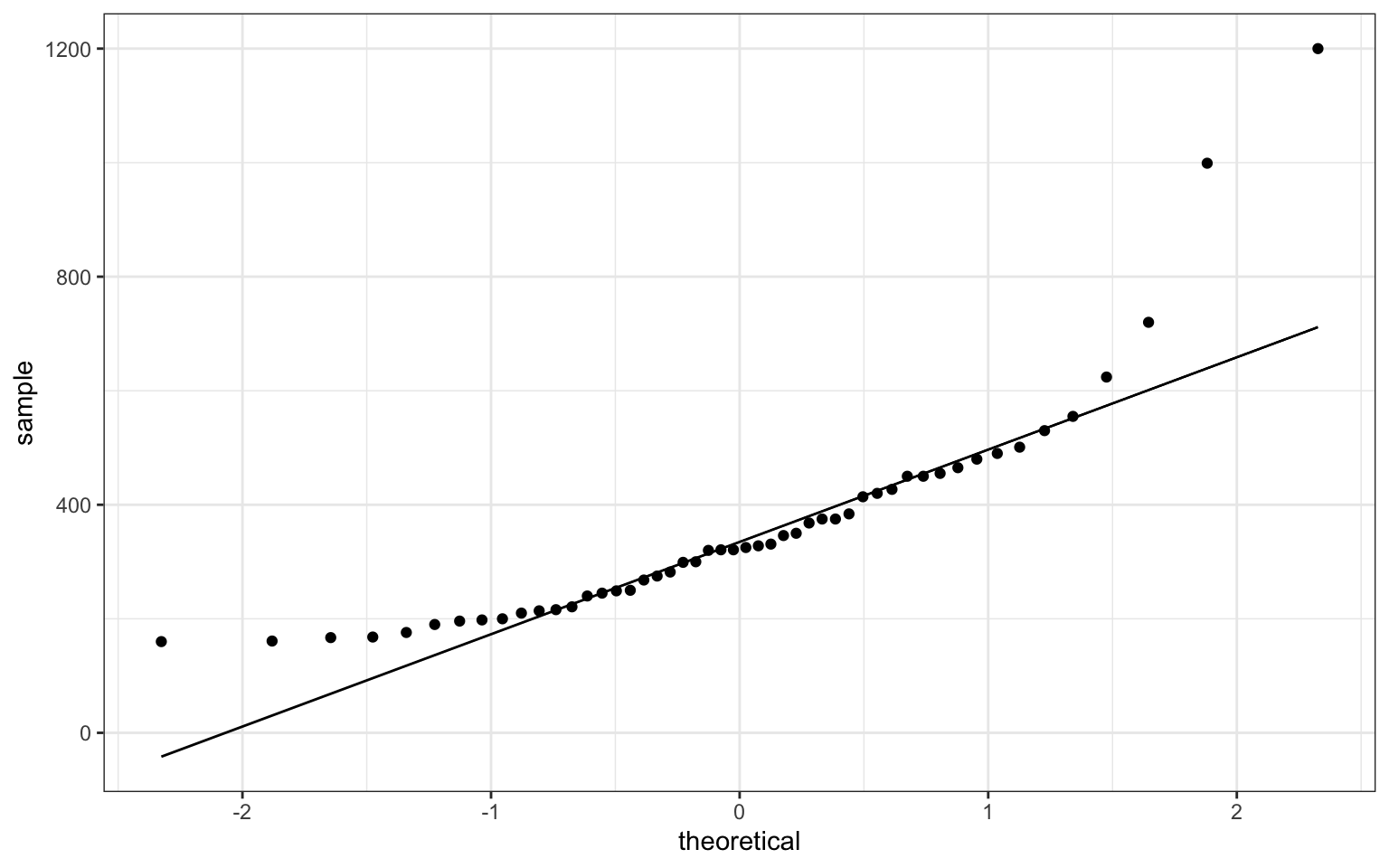

Why are the guesses not normally distributed?

Some form of bias is afoot!

It turns out that Kao et al. did an in-depth look at bias in visual estimation tasks, and it’s possible to characterize it and correct for it:

https://royalsocietypublishing.org/doi/full/10.1098/rsif.2018.0130

Here, we measure individual biases and social influence rules in multiple experiments involving hundreds of individuals performing a classic numerosity estimation task. We first investigate how existing aggregation methods, such as calculating the arithmetic mean or the median, are influenced by these sources of error. We show that the mean tends to overestimate, and the median underestimate, the true value for a wide range of numerosities.

The authors found that the crowd consistently provides data that is non-normally distributed. The distibution of the guesses is such that the crowd overestimates when judged by the mean, but underestimates when judged by the median.

The authors went on to calculate a correction that worked quite well. They also looked at the influence of knowing others' guesses on the crowd's estimation accuracy.

In contrast to Kao et al.’s modern study, Galton’s data showed that the crowd’s median guess was just slightly high.

Let’s look at the mean and median from the current contest:

mean(guessDf$guess)

## [1] 364.18

median(guessDf$guess)

## [1] 323

Remember, the true number was 723.

The fact is that the crowd failed pretty miserably in this contest, but a couple of individuals did very well.

What do you think explains the bias in the wisdom of the crowd in our contest?